Solar 설치

홈페이지

http://www.solar-eclipse-genetics.org/

설명

Heritability 분석을 위한 프로그램이다.

1. 이 링크(https://www.nitrc.org/frs/?group_id=558)에 들어가 아래 압축 파일을 다운받는다.

SOLAR Eclipse General Version 8.1.1

2. 다운 받은 압축 파일의 압축을 푼다.

tar -zxvf 파일명.tar.gz -C /원하는위치

3. 아래 명령어로 인스톨 한다. 

./install_solar <solar-base> <solar-script-dir>

파라미터에 대한 설명 (readme 파일 열어보면 나옴)

<solar-base> is the directory name where the bulk of this release of SOLAR

is to be installed.  To keep it separate from other releases, the release

number should be included in this directory name.  For example, we use:

/opt/appl/solar/8.1.1

<solar-script-dir> is the existing directory to which the 'solar' script

that starts SOLAR is to be put.  /usr/local/bin is a typical choice.

This should be in the PATH of everyone who will use solar.

You can move this script later if desired.  If you already have an older

script named 'solar' there, you must rename or delete it first.

이 때 solar-base에는 실제 실행 파일이 위치한 곳, solar-script-dir에는 실행파일을 연결할 파일의 경로를 써준다. 일반적으로 solar-script-dir은 /usr/local/bin 파일에 위치하도록 하고, solar-base는 아무 곳에나 놔두어도 되지만 /usr/local/bin에 위치해도 크게 상관은 없다. 

***********************************************************

Ignore error messages (if any) from the tests below

Ignore error messages (if any) from the tests above

***********************************************************

    *** Successful Installation ***

SOLAR has been installed with the command name solar

The new documentation directory is /mnt/c/Users/JuYoungAhn/Downloads/solar/8.1.1/doc

For command line editing, give command ./install_rlwrap

root@DESKTOP-F14K9HF:/mnt/c/Users/JuYoungAhn/Downloads/solar_linux# solar

/mnt/c/Users/JuYoungAhn/Downloads/solar/8.1.1/bin/rlwrap: 1: /mnt/c/Users/JuYoungAhn/Downloads/solar/8.1.1/bin/rlwrap: Syntax error: "(" unexpected

SOLAR Eclipse version 8.1.1 (General), last updated on January 29, 2018

Copyright (c) 1995-2018 Texas Biomedical Research Institute

Enter help for help, exit to exit, doc to browse documentation.

위와 같은 메시지가 뜨면 설치 완료된 것이고, /usr/local/bin에 script 파일을 넣은 경우 환경변수를 설정하지 않아도 커맨드 창에 solar를 치면, solar가 실행된다.

False Discovery Rate

False Discovery Rate(FDR)는 다중비교문제에서 1종 오류를 조절하는 방법이다. FDR은 특히 유전학 연구에서 대량의 유전체 마커와 질병과의 연관성을 보는 연구(예를 들어 Genome-wide association study)에서 많이 사용하는 방법이다.

다중비교문제에서 기본적으로 많이 사용하는 본페로니 방법은 전체 테스트의 1종 오류를 alpha (예를 들어0.05)로 고정하는 방법이다. 즉, 전체 테스트가 유의하지 않은데 유의하다고 잘못판단할 확률을 0.05로 한다는 것이다.

50000개의 마커에 대해 연관성을 검정하며,  이 중 49000개가 실제로 연관성이 없고, 나머지 1000개가 실제 연관성이 있다고 해보자.

개별 테스트의 1종 오류를 0.05로 고정하면, 1종 오류는 유의하지 않은데, 유의하다고 판단할 확률이므로 49000*0.05 = 2450개가 평균적으로 false positive가 된다. 즉, 49000개 중에 2450개를 유의하다고 잘못판단하고, 나머지 46550개를 유의하지 않다고 잘 판단한 것이다. 만약 1000개의 실제 연관성이 있는 마커중 900개를 유의하다고 판단하고, 100개를 유의하지 않다고 판단했다고 하면, 총 3350개를 유의하다고 판단해서 그 중에 900개가 맞은 것이다.

본페로니 보정을 이용하여 전체 테스트의 1종 오류를 0.05로 고정하면 개별 테스트의 컷오프는 0.05/50000이 되므로, 49000*0.05/50000 = 약 0.05가 평균적으로 false positive가 된다. 따라서 본페로니 보정을 이용하면 false positive를 확연히 줄일 수 있다. 하지만 본페로니 보정의 단점은 너무 컷오프가 엄격하기 때문에 실제 유의한 마커의 effect size가 크지 않은 경우 유의하지 않다고 판단할 수 있다는 것이다. 이것이 소위 말하는 power의 문제이며, 1종 오류와 2종 오류가 trade off 관계임을 알 수 있다. 이렇게 false positive를 엄격하게 통제하면 너무 보수적인 결정을 내리게 되며 실제 유의한 마커를 찾아내기가 힘들어진다. 따라서 어느정도의 오차를 허용하면서 실제 유의한 마커도 잘 골라내는 방법이 필요하게 된다.

따라서 이러한 연구에서는 False Discovery Rate, 즉 유의하다고 판단한 것중에 틀릴 확률을 고정시키는 새로운 p-value를 정의하는 방법을 많이 사용한다. 우선 FDR의 정의부터 보면,

FDR = false positive / total positive (total positive = false positive + true positive)

즉, 유의하다고 판단한 것 중에 실제로는 유의하지 않은 것의 비율이다. 이 비율을 0.05로 고정한다면, 유의하다고 판단했을 때 틀릴 확률은 0.05로 고정할 수 있다. 이는 위의 접근법과는 다소 다르다. 1종 오류는 유의하지 않은데 유의하다고 판단할 확률이지만, FDR은 유의하다고 판단했을 대, 이것이 틀릴 확률이다. 위의 경우에는 3350개를 유의하다고 판단했는데 이 중 틀린 것이 2450이므로 FDR = 2450/3350 = 0.73 이다. 수많은 false positive로 인해 FDR이 높아졌음을 알 수 있고, 데이터가 밸런스하지 않기 때문에 실제 유의한 마커를 찾는 것이 매우 힘들다는 것을 알 수 있다.

근데 FDR은 실제 정답을 알아야 알 수 있다. 실제 유의한 (혹은 인과적 관계를 갖는) 마커를 알아야 FDR을 정확히 구할 수 있는데 이것은 힘든 일이다. 따라서 다양한 방법으로 FDR을 추정하는데 대표적인 방법으로는 Benjamini-Hochberg procedure가 있다.

위키피디아의 정의를 보자.

Benjamini–Hochberg procedure

The Benjamini–Hochberg procedure (BH step-up procedure) controls the FDR at level ${\displaystyle \alpha }$.^[1] It works as follows:

1. For a given ${\displaystyle \alpha }$, find the largest k such that ${\displaystyle P_{(k)}\leq {\frac {k}{m}}\alpha .}$
2. Reject the null hypothesis (i.e., declare discoveries) for all ${\displaystyle H_{(i)}}$ for ${\displaystyle i=1,\ldots ,k}$.

우선, 모든 마커의 p-value를 큰 것부터 작은 것으로 내림차순 정렬을 한 후, 개별 테스트의 p-value를 각각 다르게 적용시키는 방법이다. 예를 들어, alpha = 0.05, m=50000, k=50000 인 경우, 가장 p-value가 큰 마커이다. 이 마커의 경우 p-value의 기각역은 50000*0.05/50000 = 0.05 이다. 즉, p-value가 낮은 마커로 갈 수록 점점 엄격한 p-value의 컷오프를 적용한다. Benjamini-Hochberg procedure는 이러한 방식으로 FDR을 0.05로 고정한다.

# 2018.2.6 추가

Benjamini 방법을 통해 기각역을 정하는 것을 시각화해서 보면 위와 같은 그림이 된다. 기각역을 고정시키는 본페로니나 Holm's의 방법(회색선) 보수적인 기각역을 갖고, FDR의 경우(빨간색선) 어느 정도 false positive를 허용함으로써 너무 보수적이지 않도록 기각역을 조정한다.

참고 : http://t-lab.tistory.com/28

어떻게 세포는 자신들이 필요한 유전자를 발현 시킬까?

위에서는 유전자가 단백질로 변화하는 과정 속에서 유전자 조절이 언제 이루어지는지 알아보았습니다. 그렇다면 구체적으로 어떻게 세포는 원하는 유전자만 발현시켜 원하는 기능을 수행할 수 있을까요? 이는 각각의 세포들이 제각기 다른 전사 조절 인자들을 갖고 있기 때문입니다. 이러한 조절 인자들은 전사를 촉진(activate)시키기도 하고 방해(repress)하기도 합니다. 전사 조절 인자는 단백질이며, 이 전사조절인자도 유전자들이 코딩하고 있습니다.

일반적으로 전사는 RNA 중합효소가 소위말하는 프로모터 시퀀스에 결합함으로써 시작됩니다. 이 시퀀스는 전사 시작 지점에 근접한 upstream 방향에 존재합니다. (5' 쪽 방향) 하지만 downstream 방향에도 존재할 수 있습니다. (3' 쪽 방향) 비교적 최근에 연구자들은 인핸서 시퀀스라는 것을 발견하였습니다. 인핸서는 전사 조절 단백질들이 결합할 수 있는 결합 위치(binding site)를 제공함으로써 전사에서 중요한 역할을 하는 시퀀스입니다. 이 인핸서의 전사 조절 단백질이 붙게되면 염색질 구조가 변화되어 RNA 중합효소나 조절 단백질의 결합을 촉진하거나 억제하는 역할을 하게됩니다. 이 때 염색질 구조를 open chromatin structure라고 하는데, 이는 유전자 전사가 활성화 된다는 것과 연관이 있습니다. 반면 염색질의 구조가 빽빽한 경우, 전사가 억제되어 있는 것과 연관이 있습니다.

몇몇 조절 단백질은 다양한 유전자의 전사에 영향을 미칩니다. 이는 전사 조절 단백질 결합 위치 (regulatory protein binding site 혹은 transcription factor binding site라고도 함)가 다양한 곳에 존재하기 때문입니다. 결과적으로 조절 단백질은 다양한 유전자의 걸쳐 다양한 역할을 합니다. 조절 단백질의 역할은 단지 어떤 한 유전자의 발현을 조절하는 것이 아니라 다양한 유전자의 발현을 조절합니다. 이것이 각각의 세포가 한 번에 많은 수의 유전자를 조절할 수 있는 하나의 메커니즘입니다.

Figure 2: 전사의 조절

활성 단백질이 인핸서 시퀀스에 결합하게되면 RNA 중합효소를 활성화 시키는 프로모터 부분에 단백질을 끌어들일 수 있고, 이로 인해 전사가 촉진된다. DNA는 위와 같이 굽어져 활성자 단백질은 RNA 중합효소의 활동을 중재하는 다른 단백질들과의 상호작용을 하게 된다.

우선 원핵 세포에 대해서 알아보면, 원핵생물에서 조절 단백질은 종종 영양소의 이용가능성에 의해 조절됩니다. 이는 박테리아와 같은 생물이 환경 조건에 반응하여 전사 패턴을 빠르게 조절할 수 있게 합니다. 덧붙여, 원핵생물의 조절 부위는 프로모터와 가깝게 위치합니다.

Figure 3: 프로모터 주위에서의 전사 조절

특정 단백질은 RNA 중합효소에 간섭을 함으로써 전사를 조절한다. 불활성화 상태로 존재하는 억제 단백질(repressor)은 다른 분자에의해 활성화 될 수 있으며, 활성화된 상탱서 operator라 불리는 부위에 결합하여 RNA 중합효소가 프로모터에 결합하는 것을 방해한다. RNA 중합효소가 프로모터 부위에 결합하여야 전사가 개시됨으로 이는 전사를 효과적으로 억제한다. 

활성자(activator)는 프로모터 주위에 조절 부위에 결합하여 RNA 중합효소의 활동을 촉진합니다. 억제자(repressor)는 조절부위에 결합하여 RNA 중합효소의 결합을 방해합니다. 

진핵생물의 유전자 발현 조절은 원핵생물에 비해 복잡합니다. 위에서 기술한 것과 마찬가지로 기본적으로는 프로모터 주위 조절 부위에 결합하는 활성자, 억제자에 의해 RNA 중합효소의 활동량이 조절되어, 전사 과정에서의 유전자 조절이 일어납니다. 하지만 진핵생물에서는 그 이상의 많은 수의 조절 단백질이 존재하며, 조절 단백질의 결합 부위는 프로머터와 멀리 떨어져 있는 경우도 많습니다. 이로 인해 유전자 발현의 조절이 더욱 유연하게 됩니다.

Figure 4: 많은 수의 전사 조절 인자

전사 조절 인자들은 각각 다른 역할을 갖고 있다. 위의 3가지 전사 조절인자는 Mediator 복합 단백질과 각각 다르게 상호작용하여 전사를 조절한다. 각각의 조절단백질이 있고 없음, 또한 이들이 어떻게 조합되느냐에 따라 유전자의 발현이 달라진다. 진핵 생물의 유전자 발현의 특징은 이러한 복합한 조절 과정을 통해 같은 유전자라도 다르게 번역될 수 있다는 것이다.

다른 세포 유형은 특징적인 전사 조절인자를 갖고 있습니다. 다세포 생물에서 다른 세포는 각각 다른 조절 인자들의 조합을 갖고 있습니다. 이로인해 각기 다른 기능을 하는 다양한 세포가 생성되고, 기능할 수 있는 것입니다.

Figure 5: 전사 조절인자가 세포 유형을 결정한다.

세포 발달 과정에 따라 전사 조절 인자가 달라지는 것을 나타내는 그림

세포 유형의 다양성은 다른 전사조절인자들의 활동에 의한 것이다.

참고 : Nature Education Gene expression

Chip-seq 데이터를 통한 binding motif의 분석

Chip-seq 을 통해 대략적인 protein binding site (혹은 histon modification)의 시퀀스를 알고, 이 시퀀스들 중에서 비슷한 시퀀스를 찾아내어 해당 protein에 specific한 시퀀스가 무엇인지를 알아내는 분석이다. 이를 수행하는 bioinformatics Tool은 매우 많으며, [Evaluating tools for transcription factor binding site prediction] 논문에서 좋은 평가를 받았던 rGADEM을 이용하여 binding motif를 찾는 분석을 해보도록 한다. rGADEM은 GADEM 방법을 r로 구현한 것이며, GADEM은 motif를 찾는데 Genetic 알고리즘과 EM 알고리즘을 결합하여 사용한다. 자세한 방법론은 본 포스팅에서 다루지 않는다. 본 포스팅은 이 튜토리얼을 참고하였다.

# rGADEM Tutorial
# reference : https://bioconductor.org/packages/devel/bioc/vignettes/rGADEM/inst/doc/rGADEM.pdf

source("https://bioconductor.org/biocLite.R")
# biocLite("rGADEM", lib="C:/Users/Documents/R/win-library/3.4")
# biocLite("BSgenome.Hsapiens.UCSC.hg19", lib="C:/Users/Documents/R/win-library/3.4")
# biocLite("DNAStringSet", lib="C:/Users/R/win-library/3.4")

# install.packages("RCurl")

library(RCurl)
library(rGADEM)
library(BSgenome.Hsapiens.UCSC.hg19)

rGADEM은 bioLite 패키지에 있으며, 위와 같이 설치할 수 있다. rGADEM, BSgenome..., DNAStringSet 3개의 bioLite 패키지를 설치한 후, 이와 의존성이 있는 RCurl 패키지까지 설치하면 라이브러리 로드가 완료된다.

데이터

Test_100.bed

Test_100.fasta

rGADEM을 설치하면 위 예제 데이터가 패키지 안에 기본으로 들어있다. 이 예제 데이터를 통해 실습을 해보도록 한다.

chipseq 데이터로 binding motif를 분석하기까지의 pipeline은 QC, peak calling 등의 과정을 거쳐야한다. 하지만 이번 분석에서는 peak calling까지 끝난 데이터로 분석을 한다고 가정한다. peak calling이 완료되면 protein binding이 많이 일어난 부분의 시퀀스를 얻어낼 수 있다. 이 데이터는 주로 BED 혹은 FASTA 파일로 주어진다.

1. 데이터가 BED 포맷인 경우

BED <- read.table("C:\\Test_100.bed",header=FALSE,sep="\t")
BED <- data.frame(chr=as.factor(BED[,1]),start=as.numeric(BED[,2]),end=as.numeric(BED[,3]))

BED

rgBED <-IRanges(start=BED[,2],end=BED[,3])
Sequences <- RangedData(rgBED,space=BED[,1])

rgBED
Sequences

> BED

chr     start       end
1  chr1 145550911 145551112
2  chr1 112321064 112321265
3  chr1 120124183 120124384
4  chr1 114560780 114560981
5  chr1   8044002   8044203
6  chr1 154708057 154708258
7  chr1  21537833  21538034
8  chr1 117197889 117198090
9  chr1  22547577  22547778
10 chr1 170982215 170982416
11 chr1 203938925 203939126
12 chr1 198607893 198608094
13 chr1 244838696 244838897
14 chr1  22613354  22613555
15 chr1  36725231  36725432

50 chr1  35024860  35025061

> rgBED
IRanges object with 50 ranges and 0 metadata columns:
           start       end     width
       <integer> <integer> <integer>
   [1] 145550911 145551112       202
   [2] 112321064 112321265       202
   [3] 120124183 120124384       202
   [4] 114560780 114560981       202
   [5]   8044002   8044203       202
   ...       ...       ...       ...
  [46]  24574361  24574562       202
  [47]  46110458  46110659       202
  [48] 114377432 114377633       202
  [49] 152657429 152657630       202
  [50]  35024860  35025061       202

> Sequences
RangedData with 50 rows and 0 value columns across 1 space
       space                 ranges   |
    <factor>              <IRanges>   |
1       chr1 [145550911, 145551112]   |
2       chr1 [112321064, 112321265]   |
3       chr1 [120124183, 120124384]   |
4       chr1 [114560780, 114560981]   |
5       chr1 [  8044002,   8044203]   |
6       chr1 [154708057, 154708258]   |
7       chr1 [ 21537833,  21538034]   |
8       chr1 [117197889, 117198090]   |
9       chr1 [ 22547577,  22547778]   |
...      ...                    ... ...
42      chr1 [221975293, 221975494]   |
43      chr1 [ 59123669,  59123870]   |
44      chr1 [ 76297843,  76298044]   |
45      chr1 [188010599, 188010800]   |
46      chr1 [ 24574361,  24574562]   |
47      chr1 [ 46110458,  46110659]   |
48      chr1 [114377432, 114377633]   |
49      chr1 [152657429, 152657630]   |
50      chr1 [ 35024860,  35025061]   |

2. GADEM 실행

gadem <- rGADEM::GADEM(Sequences,verbose=1,genome=Hsapiens)

interation을 돌며 GADEM 알고리즘이 실행된다.

총 2개의 motif 가 생성되었다.

> length(gadem@motifList)
[1] 2

이 중에서 첫 번째 motif는 아래와 같이 생겼다.

plot(gadem@motifList[[1]])

> gadem@motifList[[1]]@alignList
[[1]]
An object of class "align"
Slot "seq":
[1] "GCCCCGACCTCTTATCTCTG"

Slot "chr":
[1] "chr1"

Slot "start":
[1] 43552181

Slot "end":
[1] 43552382

Slot "strand":
[1] "+"

Slot "seqID":
[1] 38

Slot "pos":
[1] 100

Slot "pval":
[1] 2.209965e-09

Slot "fastaHeader":
[1] 38


[[2]]
An object of class "align"
Slot "seq":
[1] "ACCCCAACCTCTTATCTCTG"

Slot "chr":
[1] "chr1"

Slot "start":
[1] 43552181

Slot "end":
[1] 43552382

Slot "strand":
[1] "+"

Slot "seqID":
[1] 38

Slot "pos":
[1] 58

Slot "pval":
[1] 2.365196e-09

Slot "fastaHeader":
[1] 38


[[3]]
An object of class "align"
Slot "seq":
[1] "ACCCCAACCCCTTATTTCTG"

Slot "chr":
[1] "chr1"

Slot "start":
[1] 43552181

Slot "end":
[1] 43552382

Slot "strand":
[1] "+"

Slot "seqID":
[1] 38

Slot "pos":
[1] 121

Slot "pval":
[1] 5.472386e-09

Slot "fastaHeader":
[1] 38

GADEM 알고리즘은 이 motif를 설명할 수 있는 총 26개의 시퀀스를 찾았다. 이 중 3개의 시퀀스가

GCCCCGACCTCTTATCTCTG
ACCCCAACCTCTTATCTCTG
ACCCCAACCCCTTATTTCTG

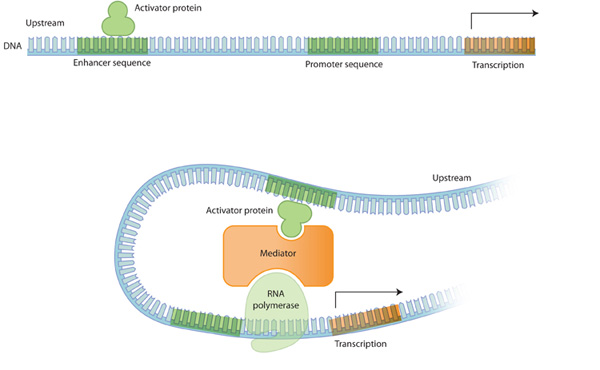
이다. 이러한 비슷한 시퀀스를 tfbs 라고 하며, tf protein이 이 곳에 달라붙어 regulatory role을 수행하게 된다.

[[26]]
An object of class "align"
Slot "seq":
[1] "CCTTCCTTCCTTTCTTCCTT"

Slot "chr":
[1] "chr1"

Slot "start":
[1] 200254533

Slot "end":
[1] 200254734

Slot "strand":
[1] "-"

Slot "seqID":
[1] 36

Slot "pos":
[1] 193

Slot "pval":
[1] 0.0001878598

Slot "fastaHeader":
[1] 36

위 결과처럼 - strand의 결과도 볼 수 있는데, 이 경우에는 BED파일에서 reverse strand를 보면 된다. 하지만 위 결과는 자동으로 reverse strand를 보여준다. http://genome.ucsc.edu/cgi-bin/das/hg19/dna?segment=chr1:200254533,200254734를 확인하면 위 시퀀스의 reverse인 aaggaagaaaggaaggaagg 를 확인할 수 있다.

3. INPUT이 FASTA 파일인 경우

# 2. Input이 FASTA 파일일 경우
path <- system.file("extdata/Test_100.fasta", package="rGADEM")
FastaFile <- paste(path,sep="")
Sequences <- readDNAStringSet(FastaFile, "fasta")
Sequences

Fasta파일의 경우 위와 같이 전처리 하면 되며, 이후의 절차는 BED 파일과 동일하다.

> Sequences
  A DNAStringSet instance of length 49
     width seq                                                                                                      names               
 [1]   202 CTACAGCTGTTCCTTGTCATCAGCCTGGGGGTGGGTAGTATTTTGATCTTA...GTCCCCATGTGACTGTAGGGTTCCTGAAACCTGGCAGGCCACTCTGCTTG FOXA1 _ 1
 [2]   202 TTATTCTGATGTGGTTTTGCGGTTATACAGTAAGCAGCACTGCTTATGTGG...ACACCAGAGGCCACCAGGACCAGAATGTTTACCAATGTAGGCAGTCACTA FOXA1 _ 10
 [3]   202 AAAGGAGAAACACAGCCAAATAATAAAACAATATCTTCTGTAAGTAAAGAG...CAAAGGTGCAAAGCCCTCTTTCAGATCCATCTCCACCATTTCCCTTCAGG FOXA1 _ 11
 [4]   202 TGTACCCCCCCAATATTTCATGATATTTACATGTTTGCATAGTACTTTCCT...CACAGGCAGAGTCAACATTGGAACTCGGAACACTGAGCCTGGCATTCCAA FOXA1 _ 12
 [5]   202 TTTAAGACTGCCACCTGAAATCAAGTCCAGTGGCTGTTCCTGTCTTCCCGT...TTATTTAACCTTTTGCCATTAGTTTACAAGAAGACGGGTTGAGCGAGTCA FOXA1 _ 13
 ...   ... ...
[45]   202 ATTAGTTCATGCCAGGCAGGGTTTGACCAAAACCTTGGACTCACTCCTGTC...TGCTGCTGCTAAGCCAGTGAGATAGATGGTGGTTTGGAAACACCCTCATG FOXA1 _ 5
[46]   202 CCAGAGCCACCACAGCCAGGCCTCTGCGGCCAGTGTCAACAAGGGGCCAGG...TGGGGTTTTGTTTACACACCTAGGGTCACCTGAAAACACCTGCTGTTTAA FOXA1 _ 6
[47]   202 CAGATCAGAGCCTGGGAGCGGGCCATGTGCAGCTGGATGGGCAGCTGGAGG...GCCCACCCTCCTGCCTTCCCAGCCAAGGAGGGAAGGGAGCTGTGGGAGGA FOXA1 _ 7
[48]   202 GGAATGTGATTTACCCAGATAAATCATCAGCTCAAGGGACTGCTTGGAGAG...TCCAGAGCTAGACGCAGAGGAAGGGGTCAAACATGTCCACATGGAACCTG FOXA1 _ 8
[49]   202 GGCTTTTCCAAGAACAATAGTGTTCTCCTAACAAACATTCGTTCCATCAGC...GGTGTTAGGGACAGAGTCCCAGGTGGCATAAAGTCGGGTTGGTCCTTGGC FOXA1 _ 9

예제 Fasta 파일의 경우 아래와 같은 motif를 찾았고, 총 74개의 sequence가 이 consensus에 부합했다. 즉, FOXA1라는 transcription factor의 binding motif (혹은 transcription factor binding site)의 consensus를 위의 Fasta 파일의 데이터를 통해 예측해볼 수 있다.

plot(gadem@motifList[[1]])

[[72]]
An object of class "align"
Slot "seq":
[1] "CTATTGACTTT"

Slot "chr":
[1] "chr"

Slot "start":
[1] 0

Slot "end":
[1] 0

Slot "strand":
[1] "-"

Slot "seqID":
[1] 4

Slot "pos":
[1] 93

Slot "pval":
[1] 0.0001517677

Slot "fastaHeader":
[1] 4


[[73]]
An object of class "align"
Slot "seq":
[1] "ATATTTACTTG"

Slot "chr":
[1] "chr"

Slot "start":
[1] 0

Slot "end":
[1] 0

Slot "strand":
[1] "+"

Slot "seqID":
[1] 42

Slot "pos":
[1] 135

Slot "pval":
[1] 0.0001719873

Slot "fastaHeader":
[1] 42


[[74]]
An object of class "align"
Slot "seq":
[1] "CTATTTGCTGG"

Slot "chr":
[1] "chr"

Slot "start":
[1] 0

Slot "end":
[1] 0

Slot "strand":
[1] "+"

Slot "seqID":
[1] 41

Slot "pos":
[1] 53

Slot "pval":
[1] 0.0001754087

Slot "fastaHeader":
[1] 41

Gene 구성요소의 5가지 분류

1. Exon

- 폴리펩타이드를 코딩하는 DNA 서열이다.

2. Intron

- 단백질을 코딩하지 않는 DNA 서열이다. * 하지만 miRNA 등의 non-coding RNA를 코딩할 수 있는 것으로 보인다.

3. Transcription Start Site

- RNA 중합효소2(polymerase)가 붙어서 전사가 시작되는 위치이다. (RNA 중합효소2는 12개의 단백질의 중합체로 mRNA를 합성해내는 물질이다.)

4. Promoter

- Core Promoter : TATA 박스(타타 박스라고 읽음)라는 것이 있는데, 이 곳은 실제로 Transcription Factor와 기타 여러 Regulatory Protein이 실제로 붙는 곳이다. 이를 통해 50여개의 단백질 complex가 만들어지며, 이것이 실제로 trascription이 일어나는데 필요한 물질들이다.

- Upstream Promoter : transcription factor 와 기타 조절 단백질(regulatory protein)이 달라붙는 부분이다. Upstream promoter는 gene마다 갯수와 타입이 다르다. transcription factor는 붙어서 해당 유전자를 활성화하거나 비활성화한다.

Promoter는 gene expression을 "총괄" 한다고 보면 되며, 이를 Enhancer가 돕는다고 볼 수 있다. 참고로 잘 알려지지 않은 것 중에 Silencer 라는 것도 있다. 이는 Histon modification과 같은 방식으로 Promoter의 반대 기능 gene expression을 억제하는기능을 수행한다.

5. Enhancer

- 보통 upstream 또는 downstream 방향으로 수천 bp 떨어진 곳에 위치하며, (또는 gene 안에 존재할 수도 있다.) transcription factor가 달라붙게 되면 promoter 쪽으로 굽어서 유전자 발현을 조절한다. 예를 들어, promoter에게 "여기는 brain이니까 이 gene을 더 발현해라!" 라고 말하는 것으로 보면 된다.

유전체에서 유전자 발현 조절 과정 (Regulation)을 수행하는 요소를 찾는 것은 중요한데, 이러한 유전체상의 조절부위(Regulatory region)을 찾는 기본적인 원리는 이 부위에 transcription factor가 달라붙는다는 성질을 이용하여 antibody를 이용한 assay를 하는 것이다.

참고그림 - 출처 위키피디아

한국어 설명 자료

https://blog.naver.com/david6703/220973718228

Gene Regulation 관련 읽어보면 좋을 글

http://genetics.thetech.org/original_news/news14

★ https://www.nature.com/scitable/topicpage/gene-expression-14121669

https://www.khanacademy.org/science/biology/gene-regulation/gene-regulation-in-eukaryotes/a/overview-of-eukaryotic-gene-regulation

GWAS, QTL, Linkage study 셋의 차이점

Linkage Study : 가족데이터 - 멘델 유전 이용, 알려진 마커로 high-penetrance, single gene disease 멘델리안 질병에 대해서 연구

QTL : 가족데이터 - 멘델 유전 이용, polygenic & quantitative trait (ex. height)

GWAS : 인구집단 데이터 - LD를 이용, polygenic, categorical trait 둘다

출처

https://www.biostars.org/p/47725/

SAS를 통한 표본 추출

sample.csv

임의추출

코드

FILENAME REFFILE 'C:\Users\\sample.csv';

PROC IMPORT DATAFILE=REFFILE
    DBMS=CSV
    OUT=WORK.population;
    GETNAMES=YES;
RUN;

proc surveyselect data=population method=srs n=200
    out=Work.sample;
run;

결과

표본 평균 계산

코드

proc surveymeans data=sample total=1459;
    var MSSubclass;
run;

결과

• 이 때, 표본 평균의 분산 추정량은 (N-n)/N * s^2/n 으로 계산된다. (유한 모집단이기 때문에 유한모집단 수정계수를 곱한다.)
• 모분산(sigma^2)을 아는 경우에는 (N-n)/(N-1) * sigma^2/n이다.

표본 비율의 추정

코드

data new;
    set sample;
    bin=(MSZoning='RL');
run;

proc surveymeans data=new total=1459;
    var bin;
run;

결과

층화 추출법

* LotShape라는 변수를 기준으로 층화추출한다. ;

proc sort data=population;
    by MasVnrType;
run;

proc freq data=population;
    tables MasVnrType;
run;

proc surveyselect data=population method=srs n=(5,5,5,5,5)
    out=sample2;
    strata MasVnrType;
run;

R - 종속변수가 순서 척도인 로지스틱 회귀분석

다항 로지스틱 회귀분석에서 종속변수가 명목형이 아닌 순서형인 경우 분석하는 방법에 관한 포스팅입니다. 이 포스팅은 이 사이트의 튜토리얼을 보고 작성하였습니다.

라이브러리 로드

require(foreign)
require(ggplot2)
require(MASS)
require(Hmisc)
require(reshape2)

데이터 읽기

dat <- read.dta("https://stats.idre.ucla.edu/stat/data/ologit.dta")
head(dat)

> head(dat)
            apply pared public  gpa
1     very likely     0      0 3.26
2 somewhat likely     1      0 3.21
3        unlikely     1      1 3.94
4 somewhat likely     0      0 2.81
5 somewhat likely     0      0 2.53
6        unlikely     0      1 2.59

X : pared(부모중 한명이 대학 학위가 있는지 여부), public(졸업한 학교가 공립인지), gpa(학점)

Y : apply (“unlikely”, “somewhat likely”, “very likely”, 각각 1, 2, 3으로 코딩되어있음) => 대학원에 진학할 가능성

이 때 Y는 순서형 척도이다.

범주형 변수의 빈도 확인

lapply 함수를 이용해 범주형 변수의 빈도표를 확인

## one at a time, table apply, pared, and public
lapply(dat[, c("apply", "pared", "public")], table)

> lapply(dat[, c("apply", "pared", "public")], table)
$apply

       unlikely somewhat likely     very likely 
            220             140              40 

$pared

  0   1 
337  63 

$public

  0   1 
343  57 

범주형 독립변수와 종속변수 관계 파악 : 3-변수 빈도표

변수 빈도표를 통해 로지스틱 회귀분석을 하기에 앞서 예상되는 결과를 미리 확인한다.

## three way cross tabs (xtabs) and flatten the table
ftable(xtabs(~ public + apply + pared, data = dat))

> ftable(xtabs(~ public + apply + pared, data = dat))
                       pared   0   1
public apply                        
0      unlikely              175  14
       somewhat likely        98  26
       very likely            20  10
1      unlikely               25   6
       somewhat likely        12   4
       very likely             7   3

연속형 변수 분포 확인

summary(dat$gpa)

> summary(dat$gpa)
   Min. 1st Qu.  Median    Mean 3rd Qu.    Max. 
  1.900   2.720   2.990   2.999   3.270   4.000 

sd(dat$gpa)

> sd(dat$gpa)
[1] 0.3979409

연속형 독립 변수와 종속 변수와의 관계 파악

Apply에 따라 gpa가 어떻게 분포하여있는지 상자그림을 통해 확인한다. 이러한 경향을 수치화하는 것이 로지스틱 회귀분석의 목표이다.

ggplot(dat, aes(x = apply, y = gpa)) +
  geom_boxplot(size = .75) +
  geom_jitter(alpha = .5) +
  facet_grid(pared ~ public, margins = TRUE) +
  theme(axis.text.x = element_text(angle = 45, hjust = 1, vjust = 1))

지금까지는 데이터에 대해서 살펴보았고, 본격적으로 순서 척도가 종속변수인 로지스틱 회귀분석을 어떻게 하는지 알아본다.

이 때 가능한 분석방법은 꼭 순서형 척도만은 아닐 것이다. GPA만을 독립변수로하여 ANOVA를 할 수도 있고, y를 1,2,3으로 놓고 다중회귀분석을 할 수도 있다. 또 y를 순서가 없는 명목형 척도로 보고 명목형 다항 로지스틱 분석(multinomial logistic regression)을 할 수도 있을 것이다. 하지만 해당 데이터에 대해 위 분석 방법들은 가정에 맞지 않는다. 따라서 순서형 척도를 종속변수로하는 로지스틱 회귀분석(ordinal logistic regression)이 적합하다.

순서형 척도를 종속변수로하는 로지스틱 회귀분석의 중요한 가정은 회귀계수가 같다고 가정하는 것이다. y=1,2,3인 이  데이터의 경우 어떠한 변수의 변화가 1 vs 2,3의 OR에 미치는 영향과 1,2 vs 3의 OR에 미치는 영향이 같다고 가정한다. y의 범주가 3개인 경우 2개의 식이 나오면 이 두식은 회귀계수가 같고, 단지 절편만 다르다.

MASS 패키지의 polr 함수를(proportional odds logistic regession) 이용하여 순서형 변수를 종속변수로하는 다항 로지스틱 회귀분석을 해보자.

회귀식을 적어주고 summary를 통해 적합된 결과를 본다. Hess=TRUE는 optimization을 할 때 사용하는 Hessian matrix를 의미한다. (https://en.wikipedia.org/wiki/Hessian_matrix)

## fit ordered logit model and store results 'm'
m <- polr(apply ~ pared + public + gpa, data = dat, Hess=TRUE)

## view a summary of the model
summary(m)

> summary(m)
Call:
polr(formula = apply ~ pared + public + gpa, data = dat, Hess = TRUE)

Coefficients:
          Value Std. Error t value
pared   1.04769     0.2658  3.9418
public -0.05879     0.2979 -0.1974
gpa     0.61594     0.2606  2.3632

Intercepts:
                            Value   Std. Error t value
unlikely|somewhat likely     2.2039  0.7795     2.8272
somewhat likely|very likely  4.2994  0.8043     5.3453

Residual Deviance: 717.0249 
AIC: 727.0249 

결과 해석

회귀계수에 exponential을 취하면 OR(Odds ratio)이 되며 이를 통해 결과를 해석해본다.

## odds ratios
exp(coef(m))

> exp(coef(m))
    pared    public       gpa 
2.8510579 0.9429088 1.8513972 

순서척도 로지스틱 회귀분석에서 OR은 proportional OR이라고도 부른다.

• 다른 변수가 고정되어있을 때, pared=0일 때에 비하여 pared=1일 때, “very likely” vs “somewhat likely” or “unlikely”의 OR이 2.851이다.
  
• 다른 변수가 고정되어있을 때, pared=0일 때에 비하여 pared=1일 때, “very likely” or “somewhat likely” vs “unlikely”의 OR이 2.851이다.
• 이는 즉, pared=1일 때, 대학원 진학(apply)을 할 가능성이 높다는 것을 뜻한다.
• 같은 binary 변수인 public도 위와 마찬가지로 해석한다.
• 다른 변수가 고정되어있을 때, gpa가 1 증가할 때, “very likely” vs “somewhat likely” or “unlikely” Odds가 1.85배가 된다.
  
• 다른 변수가 고정되어있을 때, gpa가 1 증가할 때, “very likely” or “somewhat likely” vs “unlikely” Odds가 1.85배가 된다.

이를 식으로 표현하면

log Odds(Y=very) = 2.2039 + 1.04pared - 0.05879public + 0.61594gpa

log Odds(Y=very or somewhat) = 4.2994 + 1.04pared - 0.05879public + 0.61594gpa

• 이 때, Odds(Y=1) = P(P1/(1-P1)), Odds(Y=1,2) = P((P1+P2)/(1-P1-P2))
• log Odds 는 logit function 이라고도 부른다.
  

위 두 방정식을 풀면 P(Y=1), P(Y=2), P(Y=3) 3개의 식을 얻을 수 있다. 이 식은 X가 주어졌을 때, Y의 예측값을 구한다.

PBC 데이터를 통한 생존분석

PBC 데이터 다운받을 수 있는 사이트

http://www4.stat.ncsu.edu/~boos/var.select/pbc.html

http://www4.stat.ncsu.edu/~boos/var.select/pbc.dat.txt

데이터 구조

이 데이터는 D-penicillamine의 약효를 판단하기 위한 데이터이다. 이 약이 더 오랜시간 생존에 도움이 된다는 것을 밝히는 것이 목적이다.

id       = case number
futime   = number of days between registration and the earlier of death,
           transplantion, or study analysis time in July, 1986
status   = 0=alive, 1=liver transplant, 2=dead
drug     = 1= D-penicillamine, 2=placebo
age      = age in days
sex      = 0=male, 1=female
ascites  = presence of ascites: 0=no 1=yes
hepato   = presence of hepatomegaly 0=no 1=yes
spiders  = presence of spiders 0=no 1=yes
edema    = presence of edema 0=no edema and no diuretic therapy for edema;
          .5 = edema present without diuretics, or edema resolved by diuretics;
           1 = edema despite diuretic therapy
bili     = serum bilirubin in mg/dl
chol     = serum cholesterol in mg/dl
albumin  = albumin in gm/dl
copper   = urine copper in ug/day
alk_phos = alkaline phosphatase in U/liter
sgot     = SGOT in U/ml
trig     = triglicerides in mg/dl
platelet = platelets per cubic ml/1000
protime  = prothrombin time in seconds
stage    = histologic stage of disease

여기서 status가 0이면 해당 futime에 censoring된 자료이며, 2이면 futime에 실제로 '발생'이 이루어진 경우로 censoring이 되지 않은 자료이다. status=0,1의 경우 censoring된 자료이다. 생존분석에서는 censoring이냐 아니냐가 중요하기 때문에 이 데이터를 0=censoring,1=not censoring으로 바꾸는 작업을 해주면 좋다. 생존분석에서의 종속변수 Y는 'censoring 여부와' '어떠한 사건이 발생할 때까지의 시간'이 한 세트라고 보면 된다. 다른 여러가지 변수를 통해 이 시간을 예측하는 것이 목적이라고 할 수 있다. 이를 time to event를 예착한다고 한다.

또한 이 데이터의 경우 약이 생존에 어떤 영향을 미치는지를 알아보는 연구이므로, drug를 placebo=0, D-penicillamine=1로 재코딩해주는 것이 좋다. 이렇게 재코딩함으로써 분석할 때 해석의 이점을 볼 수 있다.

PBC 데이터 읽어오기

http://www4.stat.ncsu.edu/~boos/var.select/pbc.sas.txt

options nodate nonumber ps=2000 ls=100;
data pbc;
infile 'K:\pbc.dat.txt';
    input id futime status drug age sex ascites hepato spiders edema
            bili chol albumin copper alk_phos sgot trig platelet
            protime stage;
    age = age/365.25;
if _n_ > 312 then delete;
if status=1 then status=0;
run;
proc phreg data=pbc;
model futime*status(0)=drug age sex ascites hepato spiders edema
            bili chol albumin copper alk_phos sgot trig platelet
            protime stage;
run;

SAS를 통한 분석 (Cox Regression)

proc phreg data=pbc;
    model time*delta(0)=drug sex age stage;
run;

이 때, time은 time to event이고, delta는 0=censoing, 1=not censoring이다. (0)은 0이 censoring이라는 것을 나타내준다. 실제로 알아보고 싶은것은 drug와 time(생존시간)의 관계이고, confounding을 없애기 위해 sex, age, stage와 같은 통제변수(control variable)와 함께 분석한다.  cox coxregression에서는 계수 추정치가 log(hazard ratio)의 증가량이므로 이를 exponential 해주면, hazard ratio가 증가하는 비율을 알 수 있게 된다. 예를 들어, exp(0.04474)=1.046 이다.

근데 이를 해석하면 오히려 약을 처방할 수록, hazard가 증가한다는 결론을 얻게된다. 이러한 결론에 관한 한가지 해석은 confounding에 의한 효과라는 것이다. 약을 처방받는 사람들이 대부분 위중한 환자들이기 때문에 이러한 현상이 나타나며, 제대로된 약의 효과를 알아보기 위해서는 더 많은 통제변수가 필요할 것이다.

Cox Regression에서 생존함수 식 유도하기

https://stats.stackexchange.com/questions/270164/how-do-i-interpret-a-cox-hazard-model-survival-curve